Computing Bounds on the Local Density of States using General Constraint Descent

This notebook demonstrates the use of general constraint descent (GCD) for evaluating dual bounds, using local density of states (LDOS) maximization as the example problem. For more background on LDOS optimization and bounds, see LDOS.ipynb.

The tightest dual bound for a photonic inverse design problem is found by imposing all possible local power conservation constraints in the corresponding field optimization QCQP. Unfortunately, due to the large number of constraints, evaluating this tightest dual bound can be extremely expensive.

The basic idea of GCD is to approximate the tightest dual bound with a smaller, more manageable number of constraints. This is pursued by iteratively adding new constraints to the QCQP to tighten the bounds, and merging old constraints to keep the total number of constraints fixed.

GCD is implemented for all shared projection QCQPs in dolphindes, and this notebook demonstrates the high-level use of the available GCD functionality. For more mathematical details on GCD, see Appendix B of https://arxiv.org/abs/2504.10469.

%load_ext autoreload

The autoreload extension is already loaded. To reload it, use:
  %reload_ext autoreload

import numpy as np
import scipy.sparse as sp
import matplotlib.pyplot as plt
import time
from dolphindes import photonics, geometry

# First, let's define the relevant parameters for the simulation.

wavelength = 1.0 # Dolphindes uses dimensionless units.
omega = 2 * np.pi / wavelength
chi = 4+1e-4j # Design material
px_per_length = 40 # pixels per length unit. If wavelength = 1.0, then this is pixels per wavelength.
dl = 1/px_per_length
Npmlsep = int(0.5 / dl) # gap between design region and PML. Not required to be defined, it is just convenient.
Npmlx, Npmly = int(0.5 / dl), int(0.5 / dl) # PML size.
Mx, My = int(0.5 / dl), int(0.5 / dl) # design mask size
Dx = int(0.1 / dl) # distance from the design region to the source region.
Nx, Ny = int(Npmlx*2 + Npmlsep*2 + Dx + Mx), int(Npmly*2 + Npmlsep*2 + My) # grid size. This includes the pml layer!

cx, cy = Npmlx + Npmlsep, Ny//2

ji = np.zeros((Nx, Ny), dtype=complex) # current density
ji[cx, cy] = 1.0/dl/dl # a delta function source in 2D is approximated by amplitude 1/dl/dl so that integration int(ji)dxdy = 1.0.
design_mask = np.zeros((Nx, Ny), dtype=bool) # design mask
design_mask[Npmlx + Npmlsep + Dx: Npmlx + Npmlsep + Dx + Mx, Npmly + Npmlsep: Npmly + Npmlsep + My] = True # design mask
ndof = np.sum(design_mask) # number of degrees of freedom in the design region

chi_background = np.zeros((Nx, Ny), dtype=complex) # background material
chi_background[:, :] = 0

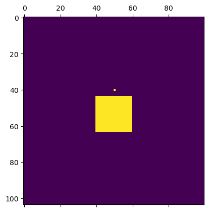
plt.matshow(design_mask + np.real(ji)*dl*dl) # visualize where the mask and the source are

<matplotlib.image.AxesImage at 0x79e75a97e9b0>

# Let's now initiate the photonics TM FDFD class. Leave the objective empty for now, let's use the class to compute the source field first.
# s0 and A0 do not have to be passed now, and in general don't need to be passed to do some EM calculations.

# Setup geometry
geometry = geometry.CartesianFDFDGeometry(
    Nx=Nx, Ny=Ny, Npmlx=Npmlx, Npmly=Npmly, dx=dl, dy=dl
)

ldos_problem = photonics.Photonics_TM_FDFD(
    omega=omega, geometry=geometry, chi=chi,
    des_mask=design_mask, ji=ji, chi_background=chi_background,
    sparseQCQP=True
)

# You can print the ldos problem to see the attributes.
print(ldos_problem)

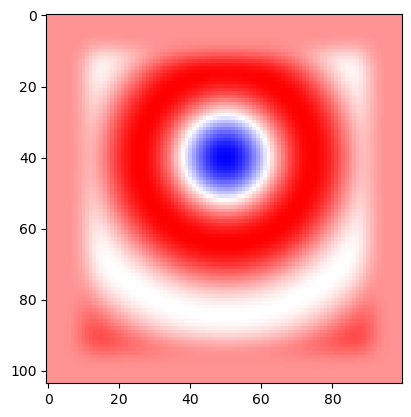
ei = ldos_problem.get_ei(ji, update=True) # update = true sets the ei to the source field. Not required if you just need to do a Maxwell solve.
plt.imshow(np.real(ei), cmap='bwr')

vac_ldos = -np.sum(1/2 * np.real(ji.conj() * ei) * dl * dl)
print("Vacuum LDOS: ", vac_ldos)

Photonics_TM_FDFD(omega=6.283185307179586, geometry=CartesianFDFDGeometry(Nx=104, Ny=100, Npmlx=20, Npmly=20, dx=0.025, dy=0.025, bloch_x=0.0, bloch_y=0.0), chi=(4+0.0001j), des_mask=True, ji=True, ei=False, chi_background=True, sparseQCQP=True)
Vacuum LDOS:  0.7878298937193577

# Now let's set s0. We need to restrict ei to the design region.
ei_design = ei[ldos_problem.des_mask] # restrict the field to the design region
c0 = vac_ldos
s0_p = - (1/4) * 1j * omega * ei_design.conj() #* dl * dl  # the dl*dl factor is not needed here, as set_objective will take care of it.
A0_p = sp.csc_array(np.zeros((ndof, ndof), dtype=complex))

# We set the objective with set_objective().
ldos_problem.set_objective(s0=s0_p, A0=A0_p, c0=vac_ldos, denseToSparse=True)

# We are ready to set up the QCQP for calculating limits. We will use Pdiags = 'global': this represents two constraints (extinction and real power global conservation). We will show how to refine these constraints below, or you may pass Pdiags = 'local' to directly do the local problem (often slower).
ldos_problem.setup_QCQP(Pdiags = 'global', verbose=1) # verbose has a few levels. 0 is silent, 1 is basic output, 2 is more verbose, 3 is very verbose.

# get a copy of the ldos_problem QCQP for testing and comparing with GCD
import copy
gcd_QCQP = copy.deepcopy(ldos_problem.QCQP)
gcd_QCQP_hs = copy.deepcopy(ldos_problem.QCQP)

Precomputed 2 A matrices and Fs vectors.

/home/alessio/code/dolphindes/dolphindes/photonics/_base_photonics.py:287: UserWarning: If both ji and ei are specified then ji is ignored.
  warnings.warn("If both ji and ei are specified then ji is ignored.")

## iterative splitting with Newton
ldos_problem.QCQP.solve_current_dual_problem(method='newton')
results = []
result_counter = 0
t = time.time()
for result in ldos_problem.QCQP.iterative_splitting_step(method='newton'): # When we reach pixel level constraints, the generator will return and stop this loop.
    result_counter += 1
    num_constr = ldos_problem.QCQP.get_number_constraints()
    print(f'at step {result_counter}, number of constraints is {num_constr}, bound is {result[0]}')

    results.append((num_constr, result[0]))
print(f'Newton iterative splitting took {time.time()-t}s to reach pixel level.')

Found feasible point for dual problem: [5.41788396e-08 1.00000000e-01] with dualvalue 816.2080132586462
Splitting projectors: 2 → Precomputed 4 A matrices and Fs vectors.
previous dual: 1.990600873418748, new dual: 1.9906008734187208 (should match)
4
at step 1, number of constraints is 4, bound is 1.9551398986638036
Splitting projectors: 4 → Precomputed 8 A matrices and Fs vectors.
previous dual: 1.9551398986638036, new dual: 1.9551398986637052 (should match)
8
at step 2, number of constraints is 8, bound is 1.8715794692206325
Splitting projectors: 8 → Precomputed 16 A matrices and Fs vectors.
previous dual: 1.8715794692206325, new dual: 1.8715794692206873 (should match)
16
at step 3, number of constraints is 16, bound is 1.86061948342903
Splitting projectors: 16 → Precomputed 32 A matrices and Fs vectors.
previous dual: 1.8564669252943178, new dual: 1.856466925294244 (should match)
32
at step 4, number of constraints is 32, bound is 1.8346626259272552
Splitting projectors: 32 → Precomputed 64 A matrices and Fs vectors.
previous dual: 1.830639882980767, new dual: 1.8306398829804047 (should match)
64
at step 5, number of constraints is 64, bound is 1.7564576543713888
Splitting projectors: 64 → Precomputed 128 A matrices and Fs vectors.
previous dual: 1.753141079194479, new dual: 1.7531410791945412 (should match)
128
at step 6, number of constraints is 128, bound is 1.6056830226992571
Splitting projectors: 128 → Precomputed 256 A matrices and Fs vectors.
previous dual: 1.6047359180016323, new dual: 1.6047359180016803 (should match)
256
at step 7, number of constraints is 256, bound is 1.5765102131704438
Splitting projectors: 256 → Precomputed 512 A matrices and Fs vectors.
previous dual: 1.572773343069001, new dual: 1.5727733430692474 (should match)
512
at step 8, number of constraints is 512, bound is 1.5557944042003922
Splitting projectors: 512 → Precomputed 800 A matrices and Fs vectors.
previous dual: 1.5547870055683592, new dual: 1.5547870055685937 (should match)
800
at step 9, number of constraints is 800, bound is 1.5454809807765972
Reached maximum projectors or pixel-level constraints.
Newton iterative splitting took 43.612792015075684s to reach pixel level.

from dolphindes.cvxopt import gcd

### now compare with tightening the bounds using GCD

## gcd parameters, play around and see how the result changes

# maximum number of QCQP constraints before merging, larger values may lead to tighter final bounds but makes GCD slower
max_cstrt_num = 10

# maximum number of GCD iterations
max_gcd_iter_num = 50

# check to see how much the bound improved after gcd_iter_period number of GCD iterations
gcd_iter_period = 5

# relative tolerance for required minimum improvement of bounds or GCD terminates
gcd_tol = 1e-2

t = time.time()

gcd_params = gcd.GCDHyperparameters(
    max_proj_cstrt_num=max_cstrt_num,
    orthonormalize=True,
    opt_params=None,
    max_gcd_iter_num=max_gcd_iter_num,
    gcd_iter_period=gcd_iter_period,
    gcd_tol=gcd_tol,
    ortho_metric="euclidean"
)
gcd_QCQP.run_gcd(gcd_params=gcd_params)
print(f'gcd took time {time.time()-t} to reach {gcd_QCQP.current_dual/ldos_problem.QCQP.current_dual} of pixel dual.')

Found feasible point for dual problem: [2.055518e-07 1.000000e-01] with dualvalue 789.381050098289
Precomputed 2 A matrices and Fs vectors.
At GCD iteration #1, best dual bound found is             1.9906008734198435.
At GCD iteration #2, best dual bound found is             1.7469384268205286.
At GCD iteration #3, best dual bound found is             1.6904015371494634.
At GCD iteration #4, best dual bound found is             1.669117289771638.
At GCD iteration #5, best dual bound found is             1.6611703027651563.
At GCD iteration #6, best dual bound found is             1.6452481749189358.
At GCD iteration #7, best dual bound found is             1.6361471371787073.
At GCD iteration #8, best dual bound found is             1.6302547947455026.
At GCD iteration #9, best dual bound found is             1.6182099497837665.
At GCD iteration #10, best dual bound found is             1.6086168530098797.
At GCD iteration #11, best dual bound found is             1.603718146915681.
At GCD iteration #12, best dual bound found is             1.589971296147006.
At GCD iteration #13, best dual bound found is             1.5853419862753348.
At GCD iteration #14, best dual bound found is             1.584176382488307.
At GCD iteration #15, best dual bound found is             1.5808257653080457.
At GCD iteration #16, best dual bound found is             1.5805080948875025.
At GCD iteration #17, best dual bound found is             1.5782609239532965.
At GCD iteration #18, best dual bound found is             1.5771810785746125.
At GCD iteration #19, best dual bound found is             1.576804060346324.
At GCD iteration #20, best dual bound found is             1.5767441307951382.
gcd took time 3.398860216140747 to reach 1.0202287510538184 of pixel dual.

# We may also use the Hilbert-Schmidt metric, which is slower per iteration but may lead to faster or better convergence
gcd_QCQP = copy.deepcopy(ldos_problem.QCQP)
t = time.time()
gcd_params = gcd.GCDHyperparameters(
    max_proj_cstrt_num=max_cstrt_num,
    orthonormalize=True,
    opt_params=None,
    max_gcd_iter_num=max_gcd_iter_num,
    gcd_iter_period=gcd_iter_period,
    gcd_tol=gcd_tol,
    ortho_metric="hilbert_schmidt"
)
gcd_QCQP_hs.run_gcd(gcd_params=gcd_params)
print(f'gcd took time {time.time()-t} to reach {gcd_QCQP_hs.current_dual/ldos_problem.QCQP.current_dual} of pixel dual.')

Found feasible point for dual problem: [6.21838174e-07 1.00000000e-01] with dualvalue 726.018736123337
Precomputed 2 A matrices and Fs vectors.
At GCD iteration #1, best dual bound found is             1.9906008743566286.
At GCD iteration #2, best dual bound found is             1.7469424006141143.
At GCD iteration #3, best dual bound found is             1.6904022844291133.
At GCD iteration #4, best dual bound found is             1.669118646168242.
At GCD iteration #5, best dual bound found is             1.6612231598651965.
At GCD iteration #6, best dual bound found is             1.6450098782106113.
At GCD iteration #7, best dual bound found is             1.633875885312799.
At GCD iteration #8, best dual bound found is             1.6269193755699332.
At GCD iteration #9, best dual bound found is             1.6169850384810138.
At GCD iteration #10, best dual bound found is             1.610662001684383.
At GCD iteration #11, best dual bound found is             1.603090291203674.
At GCD iteration #12, best dual bound found is             1.5913546683547983.
At GCD iteration #13, best dual bound found is             1.5862866331491277.
At GCD iteration #14, best dual bound found is             1.5792711288131023.
At GCD iteration #15, best dual bound found is             1.5773331231907368.
At GCD iteration #16, best dual bound found is             1.5773213500490737.
At GCD iteration #17, best dual bound found is             1.5693330528214062.
At GCD iteration #18, best dual bound found is             1.568301511814236.
At GCD iteration #19, best dual bound found is             1.564442968095412.
At GCD iteration #20, best dual bound found is             1.5655280951436892.
gcd took time 3.877166271209717 to reach 1.0129714403583396 of pixel dual.